Virtual I2K 2024: Fiji + Python

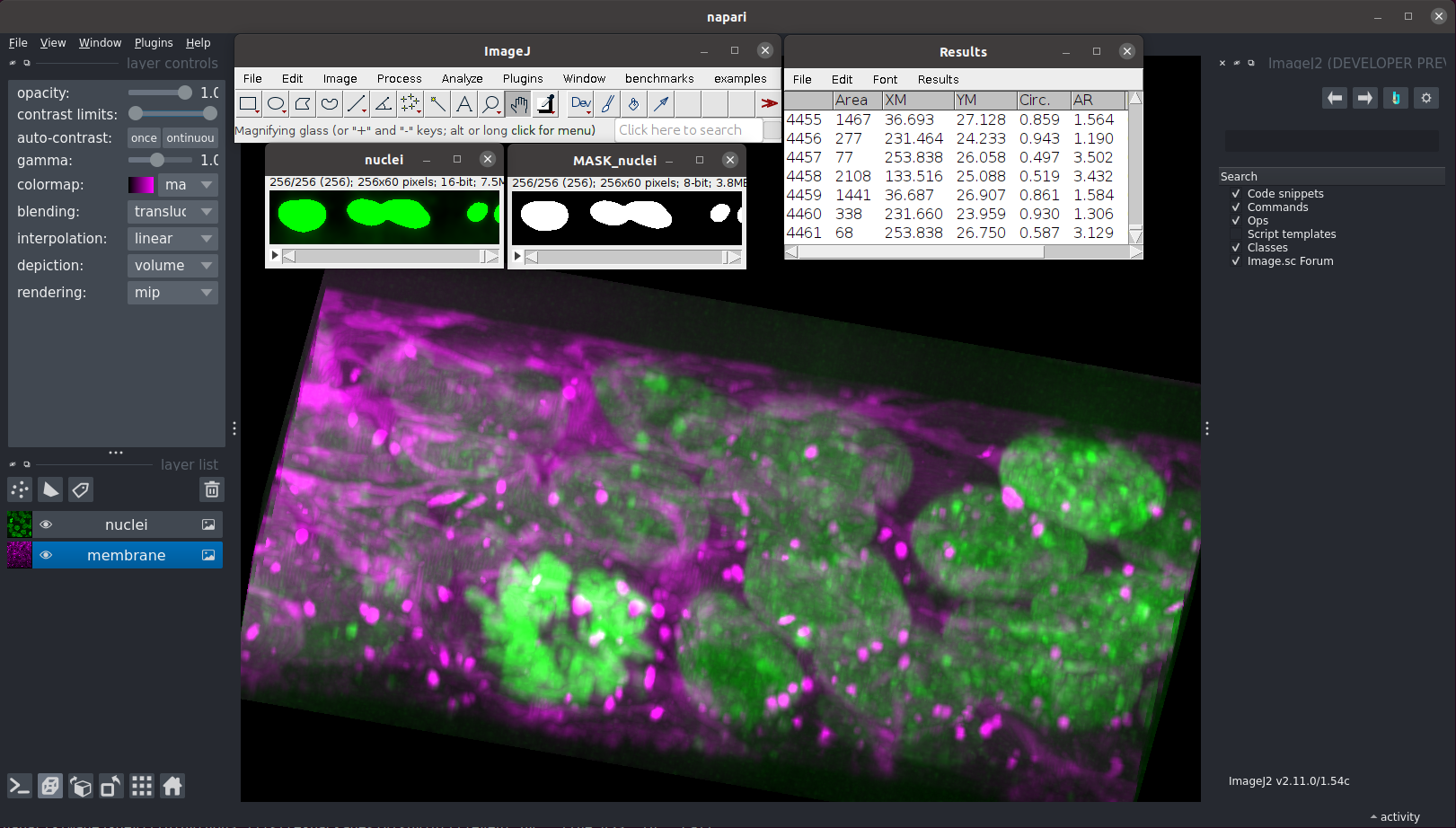
The Python software ecosystem has become a platform of choice for many image analysts, providing the Python scientific stack, deep learning toolkits, and visual tools like napari. In this workshop, you will learn how to combine Fiji with Python-based tools, including the napari user interface, as well as Python scripts, REPLs, and Jupyter notebooks. You will learn how to run Fiji/ImageJ commands such as TrackMate on input image data from napari, sending the computation results (such as images, regions of interest, and tracks) back to napari for further visualization and analysis.

This workshop assumes users:

Have existing Fiji knowledge - at a minimum, you should know what you want to do with Fiji.
Have access to mamba (Installation instructions here) on a terminal on your machine.
Have some interest in using the Python programming language.

napari and ImageJ, working side by side

Step 1: Environment Setup

This single line taken from the napari-imagej documentation will install all components necessary for this workshop, including:

Python 3.11
pyimagej, the integration layer between Fiji/ImageJ and Python
Java 8, which is necessary to run Fiji/ImageJ
napari, a popular data viewer for Python
napari-imagej, the integration layer between Fiji/ImageJ and napari

mamba create -n napari-imagej -c conda-forge python=3.11 napari-imagej=0.1.0 openjdk=8

This commmand will take a few minutes as mamba downloads and installs the components. Once it completes, you can activate the environment with:

 $ mamba activate napari-imagej

Then, create a new folder fiji-python-2024 in a convenient location - this workshop will operate within that folder.

Step 2: Create a Fiji instance!

To ensure your environment is properly set up, let's create a Python file step2.py. This file will be used to create an ImageJ2/Fiji instance, and to print the version

import imagej

ij = imagej.init()
print(f"Successfully initialized ImageJ {ij.getVersion()}")

Running the file, you should see something like the following (a different version is possible) printed out. Note that this can take up to a few minutes, depending on your internet connection, as PyImageJ downloads the latest ImageJ2:

> python step2.py
Successfully initialized ImageJ 2.16.0/1.54g

We now have an ImageJ2 instance, however it does not contain any of the plugins that come with Fiji. To obtain all of those as well, we can add a parameter to the call imagej.init() to tell PyImageJ to include Fiji as well. Note, again, that this can take up a few more minutes, as PyImageJ downloads another ImageJ version:

import imagej

ij = imagej.init("sc.fiji:fiji:2.15.0")
print(f"Successfully initialized Fiji {ij.getVersion()}")

Note the new parameter "sc.fiji:fiji:2.15.0" - it tells PyImageJ to install Fiji v2.15.0, which will get us a bunch of useful ImageJ/Fiji plugins in addition to ImageJ2/ImageJ. We'll use this Fiji installation for the rest of the workshop!

> python step2.py
Successfully initialized Fiji 2.15.0/1.54f

Tip: Interactive mode

If you want to experiment with your Fiji installation before moving on, try running python with the -i flag, which will provide you with an interactive REPL after your script finishes running. You can type exit() to quit!

$ python -i step2.py

Step 3: Data Transfer

Nearly all scientific applications in Python are built around NumPy's ndarrays, or structures that behave like them.

Unfortunately, ImageJ/Fiji has never heard of an ndarray, and instead operates on its own image structures.

Fortunately, PyImageJ provides robust API to transfer data between ImageJ/Fiji structures and ndarray structures. The subsections below describe both directions, with the end goal of blurring an ndarray in Fiji and then displaying the result in napari. Of course, your usage of Fiji may be more complicated than blurring an image, but you could replace the blurring with the Fiji behavior of your choice, and the same goes for displaying the result in napari.

Step 3.1: From Python to Fiji

If you have an image img in Python that you'd like to pass to ImageJ/Fiji, you can convert it into a Java image using the method ij.py.to_java(img). As the goal of PyImageJ is to execute Fiji functionality on data in Python, you'll need this method often.

In the script below, we can ij.py.from_java on an example image p_img. We can then blur the image using the ImageJ Ops library included in Fiji.

import imagej
import napari
from skimage.io import imread

ij = imagej.init("sc.fiji:fiji:2.15.0")

# If you have a ndarray in Python...
p_img = imread("https://media.imagej.net/workshops/data/3d/hela_nucleus.tif")

# ...you can convert it to Java...
j_img = ij.py.to_java(p_img)
# ...to do things in Fiji...
j_gaussed = ij.op().filter().gauss(j_img, 10)
print(f"Java image: {j_gaussed}")

Create a new file step3.py with the script above, and run the python file:

> python step3.py
ArrayImg [200x200x61]

Step 3.2: From Fiji to Python

The output j_gaussed from the prior script is stored within an ArrayImg, which is a data structure from ImgLib2. To convert that ArrayImg into something that we can use in Python, we can use the function ij.py.from_java(j_gaussed) transfers data in the other direction.

The script below is a continuation of the script from Step 3.1, where we convert j_gaussed into a ndarray and display it in napari:

import imagej
import napari
from skimage.io import imread

ij = imagej.init("sc.fiji:fiji:2.15.0")

# If you have a ndarray in Python...
p_img = imread("https://media.imagej.net/workshops/data/3d/hela_nucleus.tif")

# ...you can convert it to Java...
j_img = ij.py.to_java(p_img)
# ...to do things in Fiji...
j_gaussed = ij.op().filter().gauss(j_img, 10)

# ...and then convert it back to Python
p_gaussed = ij.py.from_java(j_gaussed)
# ...to do things in Python
viewer = napari.view_image(p_gaussed)

napari.run()

Replace the contents of step3.py with the script above, and run the python file:

> python step3.py

A note on `ij.py`

You'll likely find that the functions under ij.py work on many different types of data. Often times, when you're working with PyImageJ you'll see errors like:

No matching overloads found for net.imagej.ops.filter.FilterNamespace.gauss(numpy.ndarray,int), options are:
	public net.imglib2.RandomAccessibleInterval net.imagej.ops.filter.FilterNamespace.gauss(net.imglib2.RandomAccessibleInterval,net.imglib2.RandomAccessibleInterval,double)
	public net.imglib2.RandomAccessibleInterval net.imagej.ops.filter.FilterNamespace.gauss(net.imglib2.RandomAccessibleInterval,net.imglib2.RandomAccessibleInterval,double[])
	public net.imglib2.RandomAccessibleInterval net.imagej.ops.filter.FilterNamespace.gauss(net.imglib2.RandomAccessibleInterval,net.imglib2.RandomAccessibleInterval,double,net.imglib2.outofbounds.OutOfBoundsFactory)
	public net.imglib2.RandomAccessibleInterval net.imagej.ops.filter.FilterNamespace.gauss(net.imglib2.RandomAccessibleInterval,double)
	public net.imglib2.RandomAccessibleInterval net.imagej.ops.filter.FilterNamespace.gauss(net.imglib2.RandomAccessibleInterval,net.imglib2.RandomAccessible,double[])
	public net.imglib2.RandomAccessibleInterval net.imagej.ops.filter.FilterNamespace.gauss(net.imglib2.RandomAccessibleInterval,net.imglib2.RandomAccessibleInterval,double[],net.imglib2.outofbounds.OutOfBoundsFactory)
	public net.imglib2.RandomAccessibleInterval net.imagej.ops.filter.FilterNamespace.gauss(net.imglib2.RandomAccessibleInterval,double[])

In this example traceback, we can see from the first line that we tried to pass an ndarray to a method from ImageJ. Always make sure that ij.py methods are being used before and after calling ImageJ functionality!

Tip: Use xarray to preserve your metadata

If know that you always want to have metadata on your images you can use the ij.py.to_xarray() method to specify an xarray.DataArray output. This method works on both Java images and NumPy arrays, with limited support for dimension reordering.

Step 4: SciJava Scripts

ImageJ/Fiji enables reproducibility and sharing through SciJava scripts. If you've used Fiji before, you've likely written some yourself! (If you want some reading material for later, check out this guide by Albert Cardona). ij.py once again provides a mechanism, ij.py.run_script, to run any existing SciJava script.

Here, we'll utilize an existing script for Richardson-Lucy deconvolution, an algorithm that ImageJ Ops performs quite well:

#@ OpService ops
#@ ImgPlus img
#@ Integer iterations(label="Iterations", value=15)
#@ Float numericalAperture(label="Numerical Aperture", style="format:0.00", min=0.00, value=1.45)
#@ Integer wavelength(label="Emission Wavelength (nm)", value=457)
#@ Float riImmersion(label="Refractive Index (immersion)", style="format:0.00", min=0.00, value=1.5)
#@ Float riSample(label="Refractive Index (sample)", style="format:0.00", min=0.00, value=1.4)
#@ Float lateral_res(label="Lateral resolution (μm/pixel)", style="format:0.0000", min=0.0000, value=0.065)
#@ Float axial_res(label="Axial resolution (μm/pixel)", style="format:0.0000", min=0.0000, value=0.1)
#@ Float pZ(label="Particle/sample Position (μm)", style="format:0.0000", min=0.0000, value=0)
#@ Float regularizationFactor(label="Regularization factor", style="format:0.00000", min=0.00000, value=0.002)
#@output ImgPlus result

import net.imglib2.FinalDimensions
import net.imglib2.type.numeric.real.FloatType

// convert input parameters into meters
wavelength = wavelength * 1E-9
lateral_res = lateral_res * 1E-6
axial_res = axial_res * 1E-6
pZ = pZ * 1E-6

// create synthetic PSF
psf_dims = new FinalDimensions(img)
psf = ops.create().kernelDiffraction(
	psf_dims,
	numericalAperture,
	wavelength,
	riSample,
	riImmersion,
	lateral_res,
	axial_res,
	pZ,
	new FloatType()
)

// convert input image to 32-bit and deconvolve with RTLV
img_f = ops.convert().float32(img)
result = ops.deconvolve().richardsonLucyTV(img_f, psf, iterations, regularizationFactor)

You can follow the steps below to run the script:

Create a folder scripts within the current directory fiji-python-2024
Within the scripts folder, create a new file decon.groovy containing the above code.
Create a new file step4.py with the code below.

import imagej
import napari
from skimage.io import imread

ij = imagej.init("sc.fiji:fiji:2.15.0")
# If you have an image in Python...
input = imread("https://media.imagej.net/workshops/data/3d/hela_nucleus.tif")

# ...and a SciJava script...
with open("./scripts/decon.groovy", "r") as f:
    script = "".join(f.readlines())

# ...you can assign that image to the script parameter...
args = {
    "img": input
}
# ...and pass it directly to the script!
result_map = ij.py.run_script("groovy", script, args)

# Note that the result is still a Java object, so we have to convert it back to Python
result = ij.py.from_java(result_map.getOutput("result"))
# ...to do things in Python
viewer = napari.view_image(result)
# (add the original for comparison)
viewer.add_image(input, name="original")

napari.run()

By running step4.py, you should see the HeLa cell deconvolved, with less background noise and more visible internal structure:

> python step4.py

Using scripts like this maximizes portability - you can write a workflow in a single SciJava script, and it can be called from Python, and within Fiji!

Step 5: `napari-imagej`

We've used napari to display the outputs of our initial explorations into PyImageJ, but ImageJ/Fiji are also graphically accessible through napari using the napari-imagej plugin. This napari plugin was designed to remove much of the hassle involved in executing ImageJ/Fiji functionality from Python - it handles all of the data conversion, providing the appearance of pure ImageJ/Fiji integration.

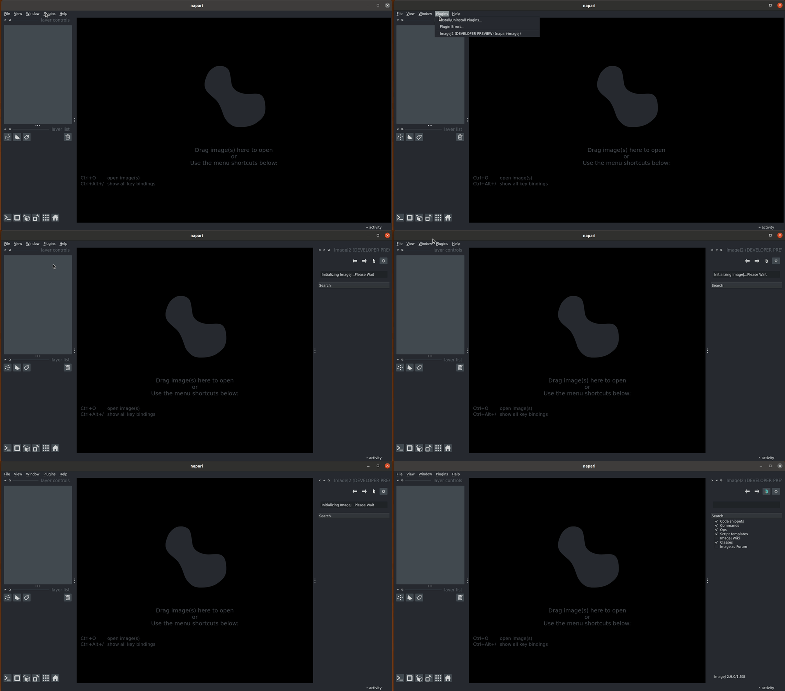
To use napari-imagej, launch napari by typing napari on your terminal. Once napari opens, go to the Plugins dropdown menu and click on the ImageJ2 (napari-imagej) menu item. napari-imagej will initialize the ImageJ2 instance for you, becoming "enabled" once the buttons become enabled.

Using napari-imagej, we have access to all* of ImageJ/Fiji, much of which now available through a seamless napari interface. As a first look at this interface, let's run the exact same gaussian blur that we ran in Step 2, using napari-imagej:

Download the image that we've been using so far: https://media.imagej.net/workshops/data/3d/hela_nucleus.tif
From your computer's Downloads folder, drag and drop the image onto the napari viewer pane.
In napari-imagej's search bar, type gauss.
Under the Ops dropdown, you'll find filter.gauss(img "out"?, img "in", number "sigma", outOfBoundsFactory "outOfBounds"?) -> (img "out"?). Double click this entry to bring up the parameter selection dialog.
For the input, select hela_nucleus, and for the sigma, enter 10. Just as we specified the out and outOfBounds parameters as optional when scripting with PyImageJ, we can leave them blank here.
Click Ok, and wait for the computation to finish. Note that in the activity pane in the bottom right hand corner of the napari window, filter.gauss will appear to notify you of its status.

Using this mechanism, you can run any ImageJ2 Command or Op, as well as any SciJava Script (as seen in the next step), using a pure napari interface, and none of the extra ij.py function calls to make everything work out!

*When we say all of Fiji, this is true for Windows and Linux - unfortunately, MacOS cannot run the UI of ImageJ/Fiji while concurrently allowing interactive access to Python or napari. This also means that MacOS users will find themselves unable to run the final section of this workshop (although we've tried to make the rest of this workshop accessible by avoiding the ImageJ/Fiji UI). This has been described in issues like this one. Many software engineers have lost many hours trying to combat this issue, but rest assured, we are still unfazed in our goal to fix it!

Step 6: Running our script again

SciJava Scripts can also be run in the napari-imagej UI. With a bit of organization, described in the steps below, we can show napari-imagej how to find these scripts:

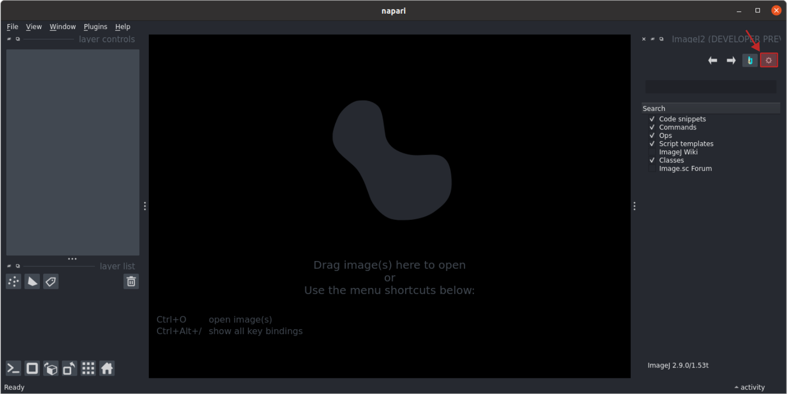
Access the settings window within napari-imagej, by clicking the "gear" icon on the right (see image below). ImageJ/Fiji needs to know which directory contains the scripts folder, (i.e. not the scripts folder itself), and so the current directory fiji-python-2024 is the one that we need to specify. Use the "ImageJ Base Directory" file chooser to set the setting to our fiji-python-2024 directory, wherever that is within your filesystem.
Restart napari and napari-imagej. On restart, ImageJ/Fiji will use this setting from napari-imagej to find our script decon.groovy.

Now that ImageJ/Fiji knows of our decon.groovy script, it will become available within the napari-imagej search results under the Commands dropdown. Follow the steps below to execute this script on our HeLa cell sample image:

If the original HeLa cell dataset is not in napari, open it as you did before, either with drag-and-drop or by selecting it in a File Browser using File->Open File(s)....
In napari-imagej's search bar, type decon.
Under the Commands dropdown, you'll find decon. Click this result twice to open the parameter selection window.
Select hela_nucleus as the img parameter, and leave all other parameters to their default setting.
Click Ok, and wait for completion to finish. While it runs, you can click the "activity" pane in napari to show current progress.

Once it finishes, you will see the deconvolved result back in napari!

Step 7: Tracking with TrackMate in `napari-imagej`

In the last step of this workshop, we will show how napari-imagej enables users to create complex workflows, using the UIs of and toolkits from both Fiji and napari. This Step is currently inaccessible to MacOS users; please see Addendum 1 for more information.

Just as we had to tell PyImageJ to run Fiji instead of just ImageJ2, we must similarly tell napari-imagej to use Fiji, which we can do by following these steps:

With napari-imagej running, click on the settings button (see image below):
Under the "ImageJ directory or endpoint" setting, enter sc.fiji:fiji:2.15.0.
Restart napari and napari-imagej.

To run TrackMate itself within Fiji, follow the tutorial here, where the process is outlined more thoroughly than we could here.

Fin

This completes the Fiji + Python workshop! Using the ideas presented in this workshop, you now know how to:

Launch and configure ImageJ/Fiji within a Python script, and in napari - note that these mechanisms work equally well in a Python REPL, or in a Jupyter Notebook
Transfer data between Python and Java equivalents, enabling the execution of ImageJ/Fiji routines on data stored in Python objects, and vice versa
How to run scripts written for ImageJ/Fiji seamlessly within a Python script, or in napari, enabling workflow distribution, portability, and reproducibility.

We hope that, using the above concepts, you can now extend the presented scripts to integrate new, exciting Python tools with your existing Fiji needs!

For more information and help, check out:

https://py.imagej.net for more information about PyImageJ
https://napari.imagej.net for more information about napari-imagej
https://forum.image.sc for interactive help about general image analysis problems - we're happy to help you resolve issues!

Addendum 1: Launching the ImageJ/Fiji UI

One of the more useful features of PyImageJ is the ability to launch and interact with the ImageJ/Fiji user interface. For accessibility, this workshop uses only "headless" (i.e. not requiring the UI) functionality with the exception of Step 7. We designed the workshop as such to maximize accessibility, as inherent limitations in MacOS limit the potential of UI display. Nevertheless, UI access is still quite powerful, and we dicuss the three flavors of UI access here.

PyImageJ offers two different mechanisms for launching a Fiji UI; users who wish to use either of these mechanisms must indicate so within the call to imagej.init:

image.init(mode="gui") tells PyImageJ to launch the ImageJ/Fiji UI and block the Python thread until the user closes it. If a user has PyImageJ installed, this is often the fastest way to launch a particular version of ImageJ/Fiji for quick experimentation.

import imagej
ij = imagej.init("sc.fiji:fiji:2.15.0", mode="gui")

image.init(mode="interactive") tells PyImageJ to launch the ImageJ/Fiji UI but returns control of the Python thread back to the user. This mechanism is unavailable on MacOS due to the threading limitations.

import imagej
ij = imagej.init("sc.fiji:fiji:2.15.0", mode="interactive")

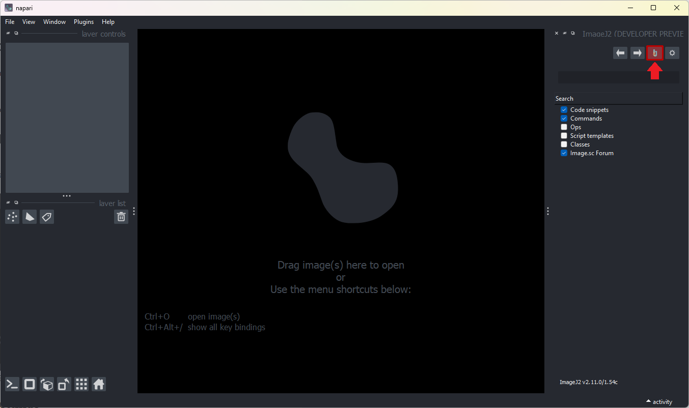
In addition, as shown in Step 7 of this workflow we can launch both the napari and ImageJ/Fiji UIs using a button within napari-imagej, using the button highlighted below. This mechanism is also unavailable on MacOS due to the threading limitations.

Addendum 2: Pitfalls in image conversion

While NumPy ndarrays provide many benefits throughout the Python ecosystem, they do not support image metadata. This means that many images stored within numpy arrays rely on dimension conventions to indicate the dimension label (e.g. X, Y, Channel, etc.). Unfortunately, these dimension conventions and lack of metadata pose three problems for Python + Fiji integration:

Python/NumPy preferred image dimensions do not align with Fiji/ImageJ.
- Python/NumPy order: (t, pln, row, col, ch) or (T, Z, Y, X, C).
- Fiji/ImageJ order: (col, row, ch, pln, t) or (X, Y, C, Z, T).
- Special care must be taken to permute/transform array shape to conform to each ecosystem's standard.
Non-standard NumPy order will be impossible to determine without additional dimension data (i.e. extra metadata indicating dimension labels).
NumPy arrays can't produce calibrated values for measurements (no metadata).

To alleviate this problem, PyImageJ offers a set of convience functions to assit in correctly converting between Python and Fiji dimension order. Notably, PyImageJ uses xarray, which supports metadata and calibrated values (i.e. the image calibration or pixel size), as the Python analog to ImageJ datasets. xarray.DataArrays (which are NumPy arrays wrapped by xarray) that have dimension labels can be properly used by PyImageJ to re-order the data into an ImageJ preferred order. Or NumPy arrays with an accompanying dimension order List can also be used with PyImageJ to indicate dimension order information. Conversely, sending data to Python with PyImageJ produces, typically, an xarray.DataArray with dimension labels and calibrated values.

For more information about PyImageJ's convenience methods, see 5 Convenience methods of PyImageJ in the PyImageJ docs. For more information about sending data to and from Python using PyImageJ, see 6 Working with Images.

Addendum 3: Jupyter Notebook

Jupyter Notebooks provide a powerful interactive setting for constructing sharable workflows, and we can utilize PyImageJ in Jupyter just as we have earlier in the workshop.

To experiment with Jupyter, we must first install it, which we can do with the following command:

$ mamba install -y -c conda-forge jupyter

We then start Jupyter, which will start a Jupyter server, opened in your default browser:

$ jupyter notebook

Create a new notebook here by selecting File->New->Notebook. Select Python 3 (ipykernel) as the kernel.

In the first cell, you can initialize an ImageJ/Fiji instance, exactly as we did before:

import imagej
ij = imagej.init("sc.fiji:fiji:2.15.0")

Jupyter users will find PyImageJ utility function ij.py.show particularly useful, as it will display an image in a matplotlib plot. This script, modified from section 3.2, can be pasted directly into the next cell.

from skimage.io import imread

ij = imagej.init("sc.fiji:fiji:2.15.0")

p_img = imread("https://media.imagej.net/workshops/data/3d/hela_nucleus.tif")
# Convert our image to Java and do stuff in Fiji
j_img = ij.py.to_java(p_img)
j_gaussed = ij.op().filter().gauss(j_img, 10)

# Then convert our image back to Python for display
gaussed = ij.py.from_java(j_gaussed)
ij.py.show(gaussed[30, :, :])

Note that ij.py.show is capable of showing images stored in both Python and Java. Can you edit the cell to have PyImageJ display the same slice without the conversion back into Python?

Addendum 4: `Mesh` visualization in napari

napari-imagej can additionally convert Fiji surface structures into napari Surface layers, providing a convenient solution for mesh/surface visualization using the napari viewer. The SciJava script written below, which converts a dataset containing a single structure in the foreground into a surface, showcases this conversion.

#@ OpService ops
#@ Img img
#@ net.imglib2.type.numeric.real.FloatType (label = "Isolevel", style = "format:0.00", min = 1.0, value = 1.0) isolevel
#@output net.imagej.mesh.Mesh output

from net.imglib2.type.logic import BitType

def apply_isolevel(image, isolevel):
    """Apply the desired isolevel on the input image.

    Apply a desired isolevel (i.e. isosurface) value on the input image,
    returning a BitType image that can be used with the marching cubes Op.

    :param image:

        Input ImgPlus.

    :param isolevel:

        Input isolevel value (FloatType).

    :return:

        An ImgLib2 Mesh at the specified isolevel.
    """
    i = isolevel.getRealDouble()
    if i > 1.0:
        i -= 1
    val = image.firstElement().copy()
    val.setReal(i)
    bin_img = ops.create().img(image, BitType())
    ops.threshold().apply(bin_img, image, val)

    return ops.geom().marchingCubes(bin_img)


output = apply_isolevel(img, isolevel)

We will run this script on this image, the same dataset used throughout the workshop. Use the following steps to set up this script for execution on the sample dataset:

Create a new file mesh.py in the scripts folder where the other scripts were placed, and copy the above script into the new file.
Start napari and napari-imagej if they are not running.
Load the dataset into the viewer if it is not loaded already.
Determine the surface isolevel, the value below which a particular location will be considered "below" the mesh. You can mouse over the image using napari to find an appropriate isolevel near the edge of the main structure.
Search for mesh in the napari-imagej search bar. The script will appear under the Commands result tab.
Double-click the mesh search result. Specify:

hela_nucleus_8_bit as the img parameter
Your determined vlaue as the isolevel parameter.

Once the script finishes, the resulting net.imagej.mesh.Mesh will be converted into a napari Surface layer and will be displayed in the viewer. You can toggle the 3D rendering capabilities of napari-imagej using a button described here.

Provide feedback

Saved searches

Use saved searches to filter your results more quickly

fiji-python-2024.md

fiji-python-2024.md

Virtual I2K 2024: Fiji + Python

Step 1: Environment Setup

Step 2: Create a Fiji instance!

Tip: Interactive mode

Step 3: Data Transfer

Step 3.1: From Python to Fiji

Step 3.2: From Fiji to Python

A note on `ij.py`

Tip: Use xarray to preserve your metadata

Step 4: SciJava Scripts

Step 5: `napari-imagej`

Step 6: Running our script again

Step 7: Tracking with TrackMate in `napari-imagej`

Fin

Addendum 1: Launching the ImageJ/Fiji UI

Addendum 2: Pitfalls in image conversion

Addendum 3: Jupyter Notebook

Addendum 4: `Mesh` visualization in napari

Files

fiji-python-2024.md

Latest commit

History

fiji-python-2024.md

File metadata and controls

Virtual I2K 2024: Fiji + Python

Step 1: Environment Setup

Step 2: Create a Fiji instance!

Tip: Interactive mode

Step 3: Data Transfer

Step 3.1: From Python to Fiji

Step 3.2: From Fiji to Python

A note on ij.py

Tip: Use xarray to preserve your metadata

Step 4: SciJava Scripts

Step 5: napari-imagej

Step 6: Running our script again

Step 7: Tracking with TrackMate in napari-imagej

Fin

Addendum 1: Launching the ImageJ/Fiji UI

Addendum 2: Pitfalls in image conversion

Addendum 3: Jupyter Notebook

Addendum 4: Mesh visualization in napari

A note on `ij.py`

Step 5: `napari-imagej`

Step 7: Tracking with TrackMate in `napari-imagej`

Addendum 4: `Mesh` visualization in napari